In logistics, the center of gravity analysis is used to derive the ideal location for warehousing facilities by calculating the transport costs to each of the supply or demand locations to be served by the facility. The center of gravity is therefore the location giving the lowest total transport costs.
From its name, it can be inferred that the center of gravity analysis is analogous to the center of mass, its physics and engineering counterpart, where the center of mass is the single point where the weighted relative position of the distributed mass sums to zero. The formula is similarly analogous with the logistics center of gravity calculated using transport volumes to and from the warehousing facility instead of distributed mass as in the physical center of mass. The formula for the coordinates of the physical center of mass or the logistics center of gravity is thus:
\[x = \frac{\sum_{i=1}^n m_i x_i }{\sum_{i=1}^n m_i}\] \[y = \frac{\sum_{i=1}^n m_i y_i }{\sum_{i=1}^n m_i}\]Where x and y refer to the coordinates of the n locations served (coordinates of the n distributed mass points for the physical center of mass) and m refers to the delivery volume (mass for the physical center of mass).
However, applying this theoretical analysis to practical problems rapidly becomes complicated as realistic assumptions and business constraints are considered, such as:
- What if there needs to be more than one warehousing facility location?
- What if the inbound and outbound shipping costs vary? This is a realistic assumption as inbound delivery costs tend to be lower since items are shipped by bulk to the warehouse and thus benefit from economies of scale while items are shipped out to customers or distributors in smaller quantities.
- What if the business only have a few candidate locations where they can set up the facility?
- How do we ensure that selected coordinates land on feasible sites for warehouse locations, e.g. the location is not in a residential area or on a mountain or on water?
For questions 1 & 2, we’ll look at how to use K-Means to get the centers of gravity. The following section includes code for implementing this in Python.
For questions 3 & 4, we will then look at how to use Itertools in Python to select the centers of gravity from a set of candidate sites. The last section includes code for implementing this.
Using K-Means for Multiple Facilities
Let’s use the following dummy data to get the centers of gravity:
| Location Name | Latitude | Longitude | Volume | Location Type |
|---|---|---|---|---|
| Manhattan, NY | 40.7831 | -73.9712 | 5,000 | Demand |
| New Haven, CT | 41.2982 | -72.9991 | 1,000 | Demand |
| Chicago, Il | 41.8333 | -88.0121 | 4,000 | Demand |
| Boston, MA | 42.3142 | -71.1103 | 3,000 | Demand |
| Raleigh, NC | 35.8436 | -78.7851 | 8,000 | Supply |
| Nashville, TN | 36.1863 | -87.0654 | 5,000 | Supply |
Suppose that we want to identify two warehouse locations using the center of gravity method. The center of mass formula from the previous section will only provide a single center of gravity, however, from its definition as the point where transport costs are minimized, we can use the K-means clustering algorithm to determine multiple locations that will minimize the transport costs as K-means clustering is an unsupervised learning technique that identifies centroids such that each individual data point is assigned a cluster based on which centroid is closest to it. To identify two warehouse locations, we can run the K-means clustering algorithm with K=2 to get two centroids that minimize the transport distances and therefore minimize the transport costs.
The code block below imports the necessary libraries for the analysis and loads the table above:
%matplotlib inline
# Import libraries
import numpy as np
import pandas as pd
import matplotlib.pyplot as plt

from itertools import combinations

from sklearn.cluster import KMeans

import folium

# Load data
data = pd.read_excel('Data.xlsx',
                     dtypes={'Location Name': str,
                             'Location Type': str})
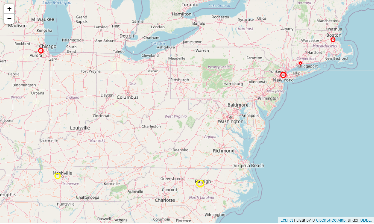
The code block below uses Folium to plot the sites (red for demand sites and yellow for supply sites) on a Leaflet map:
# Color options
color_options = {'demand': 'red',
                 'supply': 'yellow',
                 'flow': 'black',
                 'cog': 'blue',
                 'candidate': 'black',
                 'other': 'gray'}

# Instantiate map
m = folium.Map(location=data[['Latitude', 'Longitude']].mean(),
               fit_bounds=[[data['Latitude'].min(),
                            data['Longitude'].min()],
                           [data['Latitude'].max(),
                            data['Longitude'].max()]])

# Add volume points
for _, row in data.iterrows():
    folium.CircleMarker(location=[row['Latitude'],
                                  row['Longitude']],
                        radius=(row['Volume']**0.5),
                        color=color_options.get(str(row['Location Type']).lower(), 'gray'),
                        tooltip=str(row['Location Name'])+' '+str(row['Volume'])).add_to(m)
                                #row['Longitude']]).add_to(m)

# Zoom based on volume points
m.fit_bounds(data[['Latitude', 'Longitude']].values.tolist())

# Show the map
m
Also suppose that the outbound and inbound shipping costs vary, with deliveries inbound to the warehouse generally costing less for a delivery of comparable distance from the warehouse, as they tend to do due to economies of scale. Suppose that outbound deliveries cost exactly twice as much as inbound deliveries. In this case, we need to scale the weights of the volumes accordingly. The outbound deliveries to demand locations are multiplied by two while the inbound deliveries from supply locations are kept the same:
| Location Name | Latitude | Longitude | Volume | Location Type | Calc_Vol |
|---|---|---|---|---|---|
| Manhattan, NY | 40.7831 | -73.9712 | 5,000 | Demand | 10,000 |
| New Haven, CT | 41.2982 | -72.9991 | 1,000 | Demand | 2,000 |
| Chicago, Il | 41.8333 | -88.0121 | 4,000 | Demand | 8,000 |
| Boston, MA | 42.3142 | -71.1103 | 3,000 | Demand | 6,000 |
| Raleigh, NC | 35.8436 | -78.7851 | 8,000 | Supply | 8,000 |
| Nashville, TN | 36.1863 | -87.0654 | 5,000 | Supply | 5,000 |
The code block below adjusts the volumes from our raw data to account for the difference in costs between comparable inbound and outbound shipments:
# The outbound shipments cost twice as much as inbound shipments
IB_OB_ratio = 2

def loc_type_mult(x):
    """A function to get the volume multiplier based on the location type and the IB-OB ratio.
    x: The location type
    """
    if x.lower() == 'supply':
        # No need to divide since we are already multiplying the demand
        return 1
    elif x.lower() == 'demand':
        # Only apply multiplier to demand
        return IB_OB_ratio
    else:
        # If neither supply nor demand, remove entirely
        return 0

# Adjust volumes used in the computation based on IB-OB ratio
data['Calc_Vol'] = data['Location Type'].apply(str).apply(loc_type_mult)*data['Volume']
The code block below uses Scikit-learn’s implementation of the K-means clustering algorithm to get two centroids as proposed warehouse locations:
# Fit K-means for 2 centroids
kmeans = KMeans(n_clusters=2,
                random_state=0).fit(data.loc[data['Calc_Vol']>0, ['Latitude',
                                                                  'Longitude']],
                                    sample_weight=data.loc[data['Calc_Vol']>0,
                                                           'Calc_Vol'])
# Get centers of gravity from K-means
cogs = kmeans.cluster_centers_
cogs = pd.DataFrame(cogs, columns=['Latitude',
                                   'Longitude'])

# Get volume assigned to each cluster
data['Cluster'] = kmeans.predict(data[['Latitude', 'Longitude']])
cogs = cogs.join(data.groupby('Cluster')['Volume'].sum())

# Include assigned COG coordinates in data by point
data = data.join(cogs, on='Cluster', rsuffix='_COG')
The code block below plots the resulting centers of gravity using Folium on the Leaflet map, along with lines to indicate delivery routes from the proposed warehouse locations to the supply and demand sites:
# Add flow lines to centers of gravity to map
for _, row in data.iterrows():
    # Flow lines
    if str(row['Location Type']).lower() in (['demand', 'supply']):
        folium.PolyLine([(row['Latitude'],
                          row['Longitude']),
                         (row['Latitude_COG'],
                          row['Longitude_COG'])],
                        color=color_options['flow'],
                        weight=(row['Volume']**0.5),
                        opacity=0.8).add_to(m)

# Add centers of gravity to map
for _, row in cogs.iterrows():
    # New centers of gravity
    folium.CircleMarker(location=[row['Latitude'],
                                  row['Longitude']],
                        radius=(row['Volume']**0.5),
                        color=color_options['cog'],
                        tooltip=row['Volume']).add_to(m)

# Show map
m
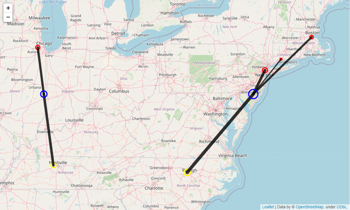
For the sample data, the algorithm appears to have selected to build the two warehouses near Urbana, Il and Wilmington, DE.
Using Itertools to Iterate Across Combinations of Sites
What if there are a limited number of locations where the warehouse can be placed? This can be due to a number of factors: the company can already own existing plots of land, or they might want to avoid getting recommendations in residential areas.
We can vary our approach by introducing candidate sites for the algorithm to select the warehouse location from. In the table below, the raw data from the previous section has been updated with five candidate sites from which to choose two warehouse locations:
| Location Name | Latitude | Longitude | Volume | Location Type |
|---|---|---|---|---|
| Manhattan, NY | 40.7831 | -73.9712 | 5,000 | Demand |
| New Haven, CT | 41.2982 | -72.9991 | 1,000 | Demand |
| Chicago, Il | 41.8333 | -88.0121 | 4,000 | Demand |
| Raleigh, NC | 35.8436 | -78.7851 | 8,000 | Supply |
| Nashville, TN | 36.1863 | -87.0654 | 5,000 | Supply |
| Boston, MA | 42.3142 | -71.1103 | 3,000 | Demand |
| Charlottesville, VA | 38.04 | -78.5199 | Candidate | |
| Harrisburg, PA | 40.3394 | -77.0077 | Candidate | |
| Columbus, OH | 39.9828 | -83.1309 | Candidate | |
| Lafayette, IN | 40.4049 | -86.9282 | Candidate | |
| Buffalo, NY | 42.8962 | -78.9344 | Candidate |
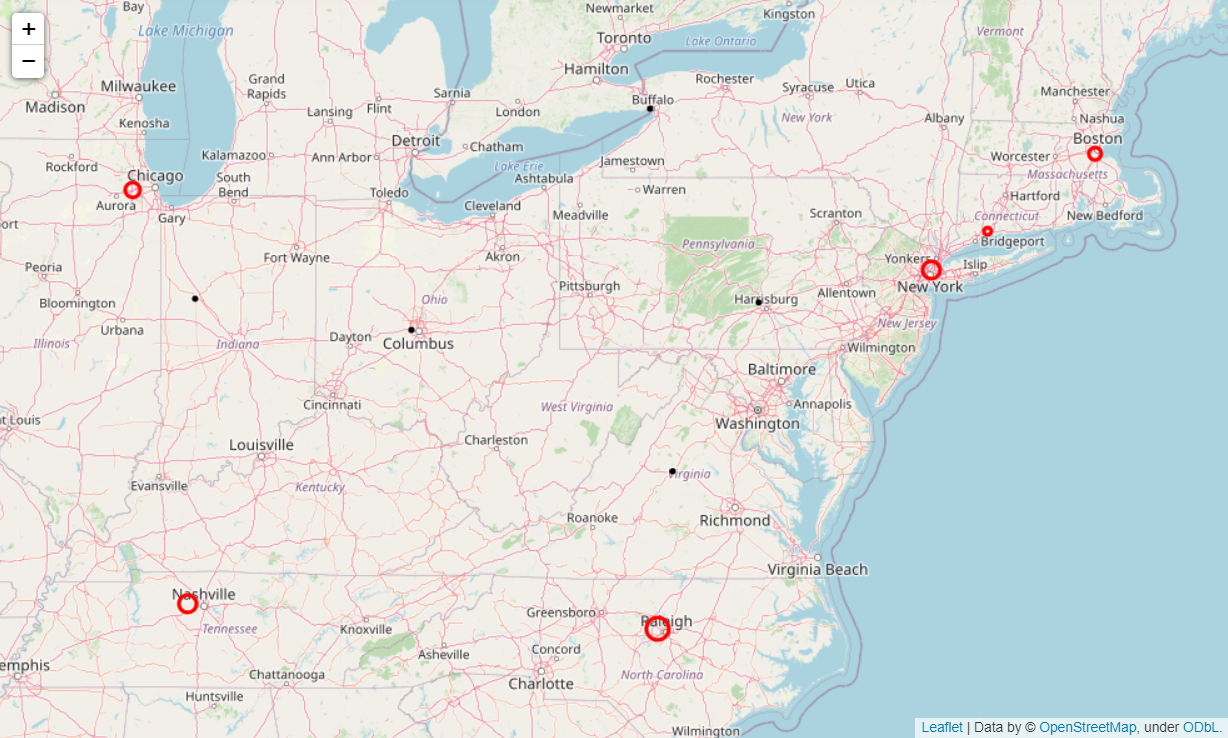
The data preparation is mostly the same and is covered by the code block below to show the supply locations (yellow) and demand locations (red) along with the candidate sites (black) in the Leaflet map:
%matplotlib inline
# Import libraries
import numpy as np
import pandas as pd
import matplotlib.pyplot as plt

from itertools import combinations

from tqdm import tqdm

from sklearn.cluster import KMeans

import folium

# Load data
data = pd.read_excel('Data.xlsx',
                     dtypes={'Location Name': str,
                             'Location Type': str})

# Color options
color_options = {'demand': 'red',
                 'supply': 'yellow',
                 'flow': 'black',
                 'cog': 'blue',
                 'candidate': 'black',
                 'other': 'gray'}

# Instantiate map
m = folium.Map(location=data[['Latitude', 'Longitude']].mean(),
               fit_bounds=[[data['Latitude'].min(),
                            data['Longitude'].min()],
                           [data['Latitude'].max(),
                            data['Longitude'].max()]])

# Add volume points
for _, row in data.iterrows():
    folium.CircleMarker(location=[row['Latitude'],
                                  row['Longitude']],
                        radius=(row['Volume']**0.5),
                        color=color_options.get(str(row['Location Type']).lower(), 'gray'),
                        tooltip=str(row['Location Name'])+' '+str(row['Volume'])).add_to(m)
                                #row['Longitude']]).add_to(m)

# Zoom based on volume points
m.fit_bounds(data[['Latitude', 'Longitude']].values.tolist())

# Show the map
m
Same as in the previous section, the code block below adjusts the volumes from our raw data to account for the difference in costs between comparable inbound and outbound shipments:
# The outbound shipments cost twice as much as inbound shipments
IB_OB_ratio = 2

def loc_type_mult(x):
    """A function to get the volume multiplier based on the location type and the IB-OB ratio.
    x: The location type
    """
    if x.lower() == 'supply':
        # No need to divide since we are already multiplying the demand
        return 1
    elif x.lower() == 'demand':
        # Only apply multiplier to demand
        return IB_OB_ratio
    else:
        # If neither supply nor demand, remove entirely
        return 0

# Adjust volumes used in the computation based on IB-OB ratio
data['Calc_Vol'] = data['Location Type'].apply(str).apply(loc_type_mult)*data['Volume']
The code block below shows a different way of solving for the centers of gravity. Itertools is used to loop through all possible combinations of warehouse locations to get the combination of n sites that will minimize transport costs. The code below calculates the total estimated transport costs based on distance weighted by relative transport costs for each combination of potential locations and saves the combination of locations that minimize this estimated cost:
cands = data.loc[data['Location Type'].str.lower()=='candidate']
locs = data.loc[data['Calc_Vol']>0]

total_dist = np.inf
best_cogs = []

# Loop to find best combination of n candidate sites (replace n with the number of sites to select)
for i in tqdm(list(combinations(cands.index, n))):
    temp_cands = cands.loc[list(i)]
    locs['Cluster'] = 0
    locs['Distance_COG'] = np.inf
    for i_l, r_l in locs.iterrows():
        for i_c, r_c in temp_cands.iterrows():
            # Get distance
            dist = (r_l['Latitude']-r_c['Latitude'])**2
            dist += (r_l['Longitude']-r_c['Longitude'])**2
            dist **= 0.5
            # Save values if distance is shorter
            if dist < locs.loc[i_l, 'Distance_COG']:
                # Save distance
                locs.loc[i_l, 'Distance_COG'] = dist
                # Save index of nearest point
                locs.loc[i_l, 'Cluster'] = i_c
    # Weight distance by volume
    locs['Weighted_Distance_COG'] = locs['Distance_COG'] * locs['Calc_Vol']
    # Save scenario if total weighted distance is smaller
    if locs['Weighted_Distance_COG'].sum() < total_dist:
        total_dist = locs['Weighted_Distance_COG'].sum()
        best_cogs = list(list(i))

# Get centers of gravity
cogs = cands.loc[best_cogs, ['Latitude',
                             'Longitude']]
# Reloop to get site assignment
locs['Cluster'] = 0
locs['Distance_COG'] = np.inf
for i_l, r_l in locs.iterrows():
    for i_c, r_c in cogs.iterrows():
        # Get distance
        dist = (r_l['Latitude']-r_c['Latitude'])**2
        dist += (r_l['Longitude']-r_c['Longitude'])**2
        dist **= 0.5
        # Save values if distance is shorter
        if dist < locs.loc[i_l, 'Distance_COG']:
            # Save distance
            locs.loc[i_l, 'Distance_COG'] = dist
            # Save index of nearest point
            locs.loc[i_l, 'Cluster'] = i_c

# Get volume assigned to each cog
cogs = cogs.join(locs.groupby('Cluster')['Volume'].sum())

# Include assigned COG coordinates in data by point
data = data.join(locs['Cluster'])
data = data.join(cogs, on='Cluster', rsuffix='_COG')
Similar to the previous section, the code block below plots the resulting centers of gravity using Folium on the Leaflet map, along with lines to indicate delivery routes from the proposed warehouse locations to the supply and demand sites:
# Add flow lines to centers of gravity to map
for _, row in data.iterrows():
    # Flow lines
    if str(row['Location Type']).lower() in (['demand', 'supply']):
        folium.PolyLine([(row['Latitude'],
                          row['Longitude']),
                         (row['Latitude_COG'],
                          row['Longitude_COG'])],
                        color=color_options['flow'],
                        weight=(row['Volume']**0.5),
                        opacity=0.8).add_to(m)

# Add centers of gravity to map
for _, row in cogs.iterrows():
    # New centers of gravity
    folium.CircleMarker(location=[row['Latitude'],
                                  row['Longitude']],
                        radius=(row['Volume']**0.5),
                        color=color_options['cog'],
                        tooltip=row['Volume']).add_to(m)

# Show map
m
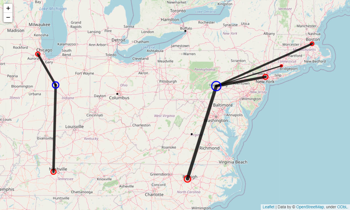
For the sample data, the algorithm has selected to build the two warehouses in Harrisburg, PA and in Lafayette, IN.
Victor Blancada is a data scientist. Visit his LinkedIn page here.