Making optimal decisions based on information from data is at the core of data science and machine learning but it is rare to find a situation where perfectly complete information is available. Oftentimes, we need to make educated guesses based on incomplete information and hopefully learn from the results of these choices to inform future decisions. To give a real life example: how can we make an informed decision on what restaurant to dine at if we have not tried every one? It is only once we have developed a sufficiently accurate model from information about the decision environment that we can make consistently the optimal choice - going back to our example, it is only after we have tried a couple of restaurants that we can make an informed decision on where to eat. However, this begs the question: When can we say that we have sufficient information? When do we stop testing different decisions?

This is the exploitation vs exploration dilemma. We need to balance testing new choices and learning new information about the decision environment (exploration) with selecting what we believe are optimal choices based on our limited choices (exploitation). Beyond our restaurant selection example, this exploitation vs exploration dilemma is encountered widely across different industries. The exploitation vs exploration dilemma exists in advertising (Which ads should we show to maximize customer response?), clinical trials (How do we ensure patient well-being while maximizing the information derived from treatment trials?), and web design (What page layouts result in higher engagement?) among others.

Mathematically speaking, the exploitation vs exploration dilemma asks us to minimize the regret we have from making bad decisions as a result of not knowing enough about the decision environment. This regret is quantified as the difference between the maximum reward from an optimal decision versus the average reward we get as a result of our current decision policy. Most approaches to the exploitation vs exploration dilemma visualize this regret using the chart below.

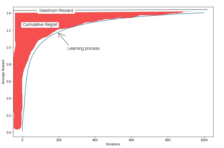
This chart displays a curve representing the learning process and plots its average reward across how many iterations or decisions it has made. The shaded area above the curve represents the cumulative regret - the gap between the average reward of the learning process and the maximum possible reward from an optimal decision. Since the goal in the exploitation vs exploration dilemma is to minimize this regret, we can infer that the ideal learning process should rise steeply during its first few iterations before leveling off at a level close to the maximum possible reward once the optimal decision policy has been estimated after a few iterations. How then do we solve the exploitation vs exploration dilemma to minimize cumulative regret during this learning process?

The multi-armed bandit is a reinforcement learning approach to solving the exploitation vs exploration dilemma. Its name is a reference to the “one-armed bandit”, a slang term for casino slot machines, since it approaches the exploitation vs exploration dilemma like selecting the slot machines which provide the highest chances of winning among a large set of slot machines with initially unknown win probabilities (hence “multi-armed bandit”, i.e. multiple one-armed bandits). In a sense, we are treating the reward coming from each choice in the decision process as a random variable of which we want to learn its distribution. In the following section, I will present a Python implementation of the multi-armed bandit approach applied to the advertising optimization problem.

I will use an advertising dataset, which you may download here. This data shows ad click rates for ten variants of an ad, where each column represents one variant of the ad and the binary values indicate whether or not a user clicked on the ad (1 for click, 0 for no click).

First, we import the required libraries. I will define the multi-armed bandit as a class, so we only need Numpy for analysis, Pandas for working with the dataset, and Matplotlib for visualization.

%matplotlib inline
# Import libraries
import numpy as np
import matplotlib.pyplot as plt
import pandas as pd

The Python class implementation of a reinforcement learning agent using the multi-armed bandit approach follows. The multi-armed bandit model is actually an entire family of algorithms and, for this case, I have implemented an agent for what is called an Upper Confidence Bound (UCB) bandit. This is designed to slowly decrease the exploration rate as more information is learned about the environment. The UCB bandit agent does this by selecting the action based on a combination of what the estimated reward is based on previous decisions plus an exploration incentive that decreases based on how many times an action has been selected before.

Where \(N_n(a)\) denotes how many times action choice \(a\) has been selected as of step \(n\) and \(c>0\) is an arbitrary constant used to control the rate of exploration.

The agent selects the action based by taking the action \(a\) which maximizes both the estimated reward \(Q_n(a)\) (exploitation) and an incentive term \(c\sqrt{\frac{log(n)}{N_n(a)}}\) that decreases as the number of times action \(a\) is selected \(N_n(a)\) increases (since the UCB bandit should not be incentivized to explore actions which it has already explored in the past).

The estimated reward \(Q_n(a)\) can be calculated in a number of ways depending on prior knowledge of the distribution of the reward function, but for this case this will simply be the sample mean of the reward from previous iterations. To make this calculation efficient as the agent runs more and more iterations, we use a formula that only requires the previous sample mean, the latest reward, and the iteration count to update the sample mean:

Where \(m_n\), the latest sample mean as of iteration \(n\), is calculated using the previous iteration’s sample mean \(m_{n-1}\),and the current iteration’s reward \(R_n\). Remember that this sample mean \(m_n\) will be used as the estimated reward \(Q_n(a)\) in the equation we had defined earlier to get \(A_n\).

# Define class for UCB bandit
class ucb_bandit:
    """Class for Upper Confidence Bound k-bandit problem 
    with a DataFrame of observations
    df: DataFrame of observations
    c: Exploration parameter (c > 0)
    iters: Number of steps (int)
    """
    def __init__(self, df, c, iters):
        """__init__ function
        """
        # DataFrame of observations
        self.df = df
        # Number of arms is the count of columns in df
        self.k = df.shape[1]
        
        # Exploration parameter
        self.c = c
        
        # Number of iterations
        self.iters = iters
        
        # Step count
        self.n = 1
        # Step count for each arm
        self.k_n = np.ones(self.k)
        
        # Total mean reward
        self.mean_reward = 0
        self.reward = np.zeros(iters)
        # Estimated reward for each arm
        self.k_reward = np.zeros(self.k)
        
    def pull(self):
        """Function to simulate pulling a bandit arm and adjust the reward estimate
        """
        # Select action according to UCB criteria (estimated reward plus exploration incentive)
        a = np.argmax(self.k_reward + self.c * np.sqrt(np.log(self.n)/self.k_n))
        
        # Return the reward randomly from the observations in df
        reward = df.iloc[np.random.randint(0, df.shape[1]), a]
        
        # Update counts
        self.n += 1
        self.k_n[a] += 1
        
        # Update total mean reward
        self.mean_reward += (reward - self.mean_reward) / self.n
        
        # Update estimated reward for arm
        self.k_reward[a] += (reward - self.k_reward[a]) / self.k_n[a]
        
    def run(self):
        """Function to iteratively run pull()
        """
        for i in range(self.iters):
            self.pull()
            self.reward[i] = self.mean_reward
            
    def reset(self):
        """Function to reset results while keeping settings
        """
        # Reset step counts
        self.n = 1
        self.k_n = np.ones(self.k)
        
        # Reset reward and reward estimates
        self.mean_reward = 0
        self.reward = np.zeros(iters)
        self.k_reward = np.zeros(self.k)

Now that the multi-armed bandit class has been defined, let’s use it to learn the optimal decision policy based on our dataset.

# Load data
df = pd.read_csv('Ads_Optimisation.csv')

We run the bandit for 10,000 iterations.

# Set UCB parameters
iters = 10000
episodes = 1000

# Initialize UCB bandit for data
ucb = ucb_bandit(df, c=2, iters=iters)

# Run UCB bandit for data for 1000 episodes

ucb_rewards = np.zeros(iters)
ucb_selection = np.zeros(df.shape[1])

for i in range(episodes):
    ucb.reset()
    
    # Run experiment
    ucb.run()
    
    # Update long-term averages
    ucb_rewards += (ucb.reward - ucb_rewards) / (i + 1)
    
    # Average actions per episode
    ucb_selection += (ucb.k_n - ucb_selection) / (i + 1)

# Plot regret during learning
plt.figure(figsize=(12, 8))
plt.plot(ucb_rewards, label='UCB', color='b')
plt.legend(bbox_to_anchor=(1.3, 0.5))
plt.xlabel('Iterations')
plt.ylabel('Average Reward')
plt.title('Average UCB Rewards after '+str(episodes)+' Episodes')
plt.show()

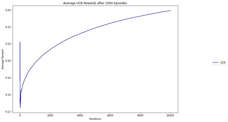
The chart above plots the average reward (i.e. clicks per ad) across iterations. We can observe that the average reward of the multi-armed bandit agent steadily increases as it learns more about the decision environment and that the average reward begins to plateau as the agent focuses on exploitation after an initial exploration period.