As developers and data scientists rise in rank and expand their scope, finance becomes an unavoidable part of their responsibilities. This post is meant to serve as a reference of basic finance formulas with annotations designed to make the formulas easier to grok for engineers.
Annual Time Value of Money
Future Value
` FV = PV(1+r)^n `
This just means that the future value of a present sum of money must be adjusted by the rate.
Present Value
` PV = (FV)/(1+r)^n `
See future value above.
Rate
` r = ((FV)/(PV))^(1/n)-1 `
The rate can be calculated by getting the ratio of the future value compared to the present value then taking its nth root, where n is the number of compounding periods (usually in years).
Years
` n = (log((FV)/(PV))) / (log(1+r)) `
The number of years can be calculated by first getting the ratio of the future value compared to the present value. Based on the previous formulas, this ratio is equivalent to one plus the rate raised by the number of compounding periods.
` (1+r)^n=(FV)/(PV)`
Take the logarithm of both sides with base (1+r).
` n*log_(1+r)(1+r)=log_(1+r)((FV)/(PV))`
` log_(1+r)(1+r)` cancels out to one and n is now isolated on the left hand side. Use the logarithm change of base rule to evaluate the right hand side.
` n = (log((FV)/(PV))) / (log(1+r)) `
Sub-Annual Time Value of Money
This section is almost exactly the same as the Annual Time Value of Money formulas except that the compounding periods are not strictly annual.
Future Value
` FV = PV(1+(r/p))^(np) `
Future Value with Continuous Compounding
` FV = PV*(e^(rn)) `
Present Value
` PV = (FV)/(1+(r/p))^(np) `
Stated Annual Rate
` r = p[((FV)/(PV))^(1/(np))-1] `
Period Rate
` r/p = ((FV)/(PV))^(1/(np))-1 `
Effective Annual Rate
` r_(effective) = (1+(r_(stated)/p))^p-1 `
Periods
` np = (log((FV)/(PV))) / (log(1+(r/p))) `
Years
` n = (log((FV)/(PV))) / (plog(1+(r/p))) `
Constant Annuity/Perpetuity
Constant Perpetuity Present Value
` PV = (PMT)/r `
Constant Perpetuity Payment
` PMT = PV*r `
Constant Annuity Present Value
` PV = ((PMT)/r)*[1-(1/(1+r)^n)] `
where n is the number of years of payments
Sub-Annual Constant Annuity Present Value
` PV = ((PMT)/(r/p))[1-(1/(1+(r/p))^(np))] `
where n is the number of years of payments and p is the number of payments per year
Constant Annuity Payment
` PMT = (PV*r)/[1-(1/(1+r)^n)] `
where n is the number of years of payments
Sub-Annual Constant Annuity Payment
` PMT = (PV(r/p))/[1-(1/(1+(r/p))^(np))] `
where n is the number of years of payments and p is the number of payments per year
Growing Annuity/Perpetuity
Growing Perpetuity Present Value
` PV = (PMT)/(r-g) `
for r>g
Growing Perpetuity Payment
` PMT = PV*(r-g) `
for r>g
Growing Annuity Present Value
` PV = (PMT)/(r-g) * [1-((1+g)/(1+r))^n] `
for r>g
where n is the number of years of payments
Sub-Annual Growing Annuity Present Value
` PV = ((PMT)/(r/p-g/p))[1-((1+g/p)/(1+r/p))^(np)] `
for r>g
where n is the number of years of payments and p is the number of payments per year
Growing Annuity Payment
` PMT = (PV*(r-g)) / [1-((1+g)/(1+r))^n] `
for r>g
where n is the number of years of payments
Sub-Annual Growing Annuity Payment
` PMT = (PV(r/p-g/p))/[1-((1+g/p)/(1+r/p))^(np)] `
for r>g
where n is the number of years of payments and p is the number of payments per year
Bonds
Present Value (Annual)
` PV = (FV)/(1+r)^n `
Present Value (Sub-Annual)
` PV = (FV)/(1+(r/p))^(np) `
Annuity Present Value (Annual)
` PV = ((PMT)/r) * [1-(1/(1+r)^n)] `
where n is the number of years of payments
Annuity Present Value (Sub-Annual)
` PV = ((PMT)/(r/p)) * [1-(1/(1+(r/p))^(np))] `
where n is the number of years of payments and p is the number of payments per year
Net Present Value
Net Present Value
` NPV = FV_0 + ((FV_1)/(1+r)) + ((FV_2)/(1+r)^2) + ((FV_3)/(1+r)^3) + … + ((FV_n)/(1+r)^n) `
Marginal Analysis
Marginal Cost
` MC_n = TC_n - TC_(n-1) `
Total Cost
` TC = VC + FC `
Average Total Cost
` ATC = (TC)/Q `
Average Variable Cost
` AVC = (VC)/Q `
Average Fixed Cost
` AFC = (FC)/Q `
Marginal Revenue
` MR_n = TR_n - TR_(n-1) `
Total Revenue
` TR = Q * p `
Marginal Profit
` MP = MR - MC ` or ` MP_n = TP_n - TP_(n-1) `
Total Profit
` TP = TR - TC `
Marginal Analysis (with Calculus)
Derivative of a Polynomial (Formulas) if y = axn then dy/dx = y’ = naxn-1
if y = a then dy/dx = y’ = 0
Derivative of a Polynomial (Term-by-Term Instructions)
- If the term is a constant then derivative is zero
- Otherwise, write sign of term
- Bring down exponent
- Multiply exponent by coefficient (the constant)
- Repeat variable (e.g., x)
- Reduce exponent by 1
- Move to step 1 for next term
Example (from lecture): y = 7x4 - 5x3 + 9x2 - 3x + 6
y’ = 47x4-1 - 35x3-1 + 29x2-1 - 13x1-1 + 0
y’ = 28x3 - 15x2 + 18x1 - 3x0
y’ = 28x3 - 15x2 + 18x - 3
Total Revenue
` TR = p * Q `
Marginal Revenue
` MR = (dTR)/(dq) `
first derivative of total revenue with respect to quantity
Total Cost
` TC = VC + FC `
Marginal Cost
` MC = (dTC)/(dq) `
first derivative of total cost with respect to quantity
Total Profit
` TP = TR − TC `
Marginal Profit
` MP = MR − MC `
or
` MP = (dTP)/(dq) `
first derivative of total profit with respect to quantity
Supply and Demand
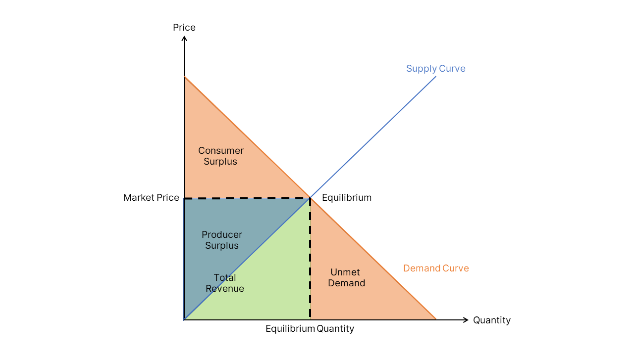
Supply Curve
A chart or formula of the relationship between price and quantity supplied by producers
Demand Curve
A chart or formula of the relationship between price and quantity demanded by consumers
Equilibrium Point
The price and quantity at which the quantity demanded is just equal to the quantity supplied. Graphically, the equilibrium point is the intersection of the supply and demand curves.
Equilibrium Quantity (q* or Q*)
The price at which the quantity demanded is just equal to the quantity supplied.
Equilibrium Price (p*)
The price at which the quantity demanded is just equal to the quantity supplied.
Market Clearing Price (p*)
Another term for equilibrium price. “Market clearing” refers to the fact that at this price all willing sellers in the market can find willing buyers and vice versa.
Total Revenue (TR)
The sum of the prices for the quantity sold. Because in most situations there is a constant market price, the total revenue is usually price times quantity. Graphically, total revenue at equilibrium is the area of the rectangle defined by the origin and the equilibrium point.
Consumer Surplus
The incremental revenue that consumers were willing to pay for a product or service but which they were able to keep because the equilibrium price is less than their willingness to pay. Graphically, the consumer surplus is the area of the triangle above the equilibrium price and below the demand curve.
Producer Surplus
The incremental revenue that producers received for a product or service above their lowest price they at which they were willing to supply. Graphically, the producer surplus is the area of the triangle below the equilibrium price and above the supply curve.
Unmet Demand
The revenue that consumers were willing to spend but didn’t because the equilibrium price is higher than their willingness to pay. Graphically, the unmet demand is the area of the triangle to the right of the equilibrium quantity and below the demand curve.
Price Elasticity of Demand
Price elasticity of demand measures the how sensitive the quantity supplied is to a change in price. Elasticity is defined as the percentage change in quantity divided by the percentage change in price.
The elasticity formula is:
` text(Elasticity) = m * (p / Q) `
where m is the slope of the demand curve equation, p is the equilibrium price, and Q is the equilibrium quantity.
Price Elasticity of Supply
Price elasticity of supply measures the how sensitive the quantity supplied is to a change in price. Elasticity is defined as the percentage change in quantity divided by the percentage change in price.
The elasticity formula is:
` text(Elasticity) = m * (p / Q) `
where m is the slope of the supply curve equation, p is the equilibrium price, and Q is the equilibrium quantity.
Basic Statistics for Finance
Median
The middle of an ordered set of values. For an even number of values, the median is the average of the two middle values of an ordered sequence.
Mode
The most frequently occurring value in a set of values. There may be more than one mode.
Range
The difference between the maximum and minimum of a set of values
Mean (Population)
` mu_x = ((sum_(i=1)^n x_i))/n `
Variance (Population)
` sigma_x^2 = ( sum_(i=1)^n(x_i-mu_x)^2 )/n `
Standard Deviation (Population)
` sigma_x = sqrt{sigma_x^2} `
Mean (Sample)
` overline{x} = (( sum_(i=1)^nx_i ))/n `
Variance (Sample)
` s_x^2 = ( sum_(i=1)^n(x_i-overline{x})^2 ) / (n-1) `
Standard Deviation (Sample)
` s_x = sqrt{s_x^2}`
Location of Quartile
` L_q = (n+1)q/4 `
where q is the quartile index (e.g., q=1 for the first quartile) and n is the number of data points.
Note: Other quartile location definitions are in common use.
Interquartile Range (IQR)
The difference between the third quartile and the first quartile of a set of values. Multiple definitions for quartile are in common use, with differences most significant for small data sets. Unlike the range, which is defined by the extreme outliers, the interquartile range captures the size of the middle 50 percent by subtracting the 25th percentile from the 75th percentile.
Location of Percentile
` L_p = (n+1)p/(100) `
Note: Other percentile location definitions are in common use.
Pearson’s Coefficient of Skewness
A statistical measure of the extent of asymmetry in a set of values. Defines skewness as a multiple of the standard deviation of a set of values. Negative values signify a data set with greater weight given to values below the median while positive values signify the opposite.
` sk_p = 3( (\text{mean}-\text{median})/(\text{standard deviation}) ) `
Excel’s SKEW Function (Sample)
A statistical measure of the extent of asymmetry in a set of values. Defines skewness as, approximately, the average cubed number of standard deviations each point falls from the mean.
` sk = n/((n-1)(n-2)) sum_(i=1)^n( (x_i- overline{x} ) /s_x)^3 `
Linear Combinations for Finance
Covariance
A statistical measure of the extent to which two variables move together above and below their respective means.
` COV_(xy) = ( sum_(i=1)^n(x_i-mu_x)(y_i-mu_y) )/n `
Note: This is a population covariance. The sample covariance would have n-1 in the denominator rather than n. This lesson uses population data.
Correlation
A normalized version of covariance with a range from -1 to +1. Positive values reflect positive correlation while negative values reflect inverse correlation, with values approaching 0 reflecting weak correlation.
` \text{Correlation} = (COV_(xy)) / (sigma_xsigma_y) `
Linear Combination
` w = ax + by `
Mean (Linear Combination)
` mu_w = amu_x + bmu_y `
Variance (Linear Combination)
` sigma_w^2 = a^2sigma_x^2 + 2abCOV_(xy) + b^2sigma_y^2 `
This formula is useful when the individual values of x and y are unknown but their variances and covariance are known.
Standard Deviation (Linear Combination)
` sigma_w = sqrt{sigma_w^2} `
Probability
Mean (from probability table)
` mu_x = sum_(i=1)^np_ix_i `
Variance (from probability table)
` sigma_x^2 = sum_(i=1)^np_i(( x_i - mu_x )^2) `
Standard Deviation
sigma_x = sqrt{sigma_x^2}
Regression
Regression is the statistical technique for finding the best line through a scatter plot of two variables. The most common form is least squares regression. “Least squares” refers to a criteria for determining the best-fit line through a two-variable data set. The criteria is to minimize the sum of the squares of the distance between each point and the line.
Regression Line
` y = mx + b `
Regression Line Slope
` m = (COV_(xy)) / (sigma_x^2) `
Regression Line Y-Intercept
` b = mu_y - m*mu_x `
Correlation
` R = (COV_(xy)) / (sigma_xsigma_y) `
A normalized version of covariance (a statistical measure of the extent to which two variables move together above and below their respective means) with a range from -1 to +1. Positive values reflect positive correlation while negative values reflect inverse correlation, with values approaching 0 reflecting weak correlation.
R-Squared
` R^2 = \text{Correlation}^2 `
A normalized version of correlation with a range from 0 to +1. R-squared, also referred to as the coefficient of determination, is the square of correlation. Values near 1 reflect strong correlation and values approaching 0 reflect weak correlation.
Normal Distribution
Uniform Distribution
A continuous probability distribution with minimum and maximum values, with all values in between of equal probability
Normal Distribution
A continuous probability distribution whose shape closely approximates the symmetrical “bell curve”. A normal distribution is completely specified by providing its mean and standard deviation.
Standard Normal Distribution
A normal distribution with mean 0 and standard deviation 1
Z-Value
The value on the standard normal distribution that corresponds to the value x on a non-standard normal distribution
X-Value
The value x on a non-standard normal distribution. In the case of a problem stated in terms of the standard normal distribution, the z-value and x-value are the same.
Normal Distribution X-to-Z Conversion
` z = (x-m)/s `
Normal Distribution Z-to-X Conversion
` x = zs+m `
Z Target Linear Interpolation
` z_(targ et) = (((p_(targ et) - p_(low))/(p_(high) - p_(low))) * (z_(high) - z_(low))) + z_(low) `